While scanning a Wikipedia article, I ran across the following formula for the matrix inverse of a matrix q:

where q _ce is an element in the c row and e column of the matrix q and the a, b element of the inverse matrix,q ^-1, is denoted q ^ab. We adopt lowered indices as a convention throughout this post.

The Levi-Civita symbol in three dimensions has the following properties:

The product of Levi-Civita symbols in three dimensions have these properties:

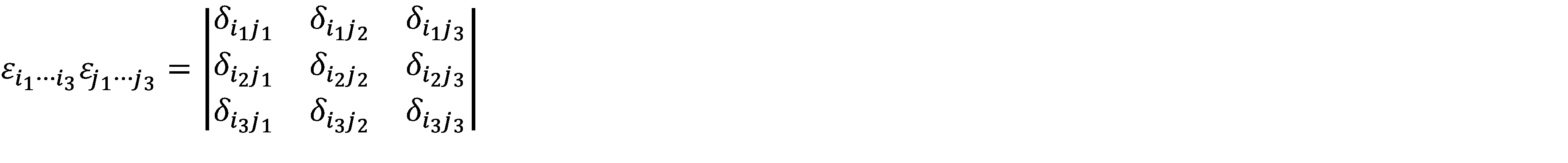
which generalizes to:

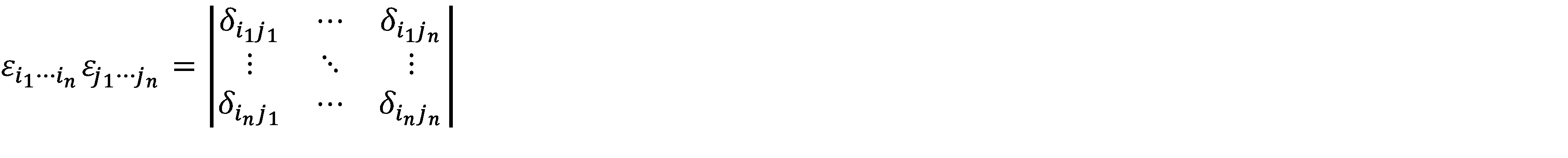
in n dimensions, where each i or j varies from 1 through n. There are n! / 2 positive and n! / 2 negative terms in the general case. Note the cyclic indicial relationships between terms and the two groupings of terms.

In both cases, the vertical bars represent the operation of taking the determinant of the enclosed matrix of Kronecker Deltas. The determinant for an arbitrary 3 by 3 matrix is:

The Kronecker Delta has these properties:

and, for any vector, a:

The determinant of a matrix A, assumed to be non-singular, has a structure similar to the inverse itself:

or, in general, assuming repeated indices are summed from 1 to n (i.e., the Einstein summation convention):

Other properties of matrix determinants are:

where the transpose of A, A^T,indicates a swap between A’s rows and columns.

Note that this implies:

and

The matrix inverse has the following properties:

and

where the adjugate, adj(A), equals the transpose of the cofactor matrix, C, which, in turn, equals the signed minor matrix M.

In index notation, we have:

In all my previous analysis, I’ve always wanted a general analytic formulation for a matrix inverse. From the notation and properties above, we have:

with Einstein summation and det(A) defined above. Another method, called the Cayley-Hamilton method, also provides an analytic expression but requires solving a linear Diophantine equation. This calculation can be expedited using the Faddeev-LeVerrier algorithm. Note that our expression involves no implicit calculations.

The expression for A ^-1  is derived starting from:

Regrouping terms, recognizing that n = δ_cc, and redefining summed indices, we get:

or

Because the matrix inverse, expressed using indices, is defined to be:

we can then make the identification:

and know that this expression for A ^-1 is unique.

From this and the adjugate definition above we see that the adjugate of A is:

The cofactors of A are:

and the minors of A are:

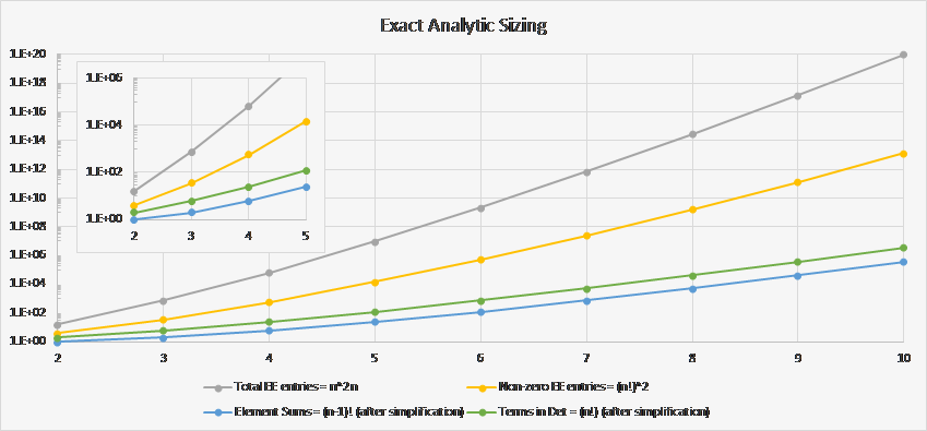
There are  n ²ⁿ elements of ɛ_i1…_1nɛ_j1…_jn, of which (n!) ² are non-zero. There are therefore ((n – 1)!) ² non-zero terms in the numerator of each matrix element A ^-1, which reduce to (n – 1)! terms after identifying like terms. There are (n!) ² terms in the determinant of A, but they reduce to n! unique terms. These generalizations are easily derived by induction from the n = 2 and 3 cases. The following graph shows how these estimates trend for n = 2 through 10:

The following graph shows that the analytic formulation is not a ready replacement for purely numerical methods used in real-time processes:

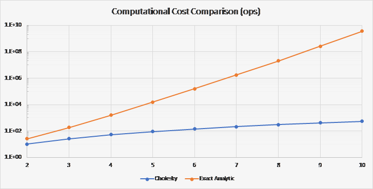
We used n ³ / 3 + 2n ² – 1/3 n for the Cholesky Decomposition method cost based on computations outlined in Numerical Recipes: The Art of Scientific Computing and n ³ n! + 2n ² + 2 for our analytic method cost.

In the Cholesky Decomposition, there are only n diagonal terms and n(n – 1) / 2 off diagonal elements that are non-zero (i.e., the other non-diagonal elements are identically zero.) The diagonal elements, in aggregate, sum n(n – 1) / 2 terms consisting of single multiplies, subtract n terms, and take n square roots. The off-diagonal terms sum, in aggregate, sum n(n – 1)(4n+ 10) / 12 terms consisting of single multiplies, subtract n(n – 1) / 2 terms, and make n(n – 1) / 2 divisions.

In the analytic method, the determinant sums two groups of n! / 2 terms, each consisting of n multiplies per term, subtracts one group from the other, and divides by a predetermined constant. Each of the n ² inverse matrix elements sum two groups of (n – 1)! / 2 terms (after identifying similar terms,) where each consists of (n – 1) multiplies per term. The inverse elements negate one of the groups, add the groups together, and divide by a constant (i.e., the previously computed determinant.)

From the two charts, the exact analytic inverse is well-suited for low dimension (  ≤ 3) analyses and modeling.

If the matrix is block decomposable, then block inversion may provide suitably small matrices with which to employ the analytic formula. Blockwise inversion is performed using either:

or

where A is square and A and (A – BD ^-1 C) ^-1 or (D – CA ^-1 B) ^-1 are non-singular. If the matrix is not square, then the Moore-Penrose pseudoinverse is appropriate.