A. Papoulis, Probability, Random Variables and Stochastic Processes

Papoulisfirst edition differs from later ones that added more contemporary subjects such as coding theory. The early text contains several equations that are useful for systems engineering modeling. The best example is the approximate formula for the variance of an arbitrary function of two random variables (7-77):

The two random variables can have any joint distribution, no assumption is made. The approximation is consistent to second order in the joint central moments. The equation is very useful to model the variance of nonlinear estimators such as a three beam bearing interpolator or an interesting detection or classification test statistic.

Papuolis documents moments for various probability distributions (pp 145 – 149, first edition). He derives Price’s theorem for moments of nonlinear functions of normal random variables (pp 226 – 228, first edition). The latter is useful for nonlinear detector analyses and other nonlinear random processes. On pages 483 – 485, he discusses the clipper correlator, once very useful (and may be so again). The text is dense but a wonderful reference for systems engineering.

C. Jakowatz, Spotlight-mode Synthetic Aperture Radar: A Signal Processing Approach

C. Jakowatz, D. Wahl, P. Eichel, D. Ghiglia, and P. Thompson have provided a valuable service to the signal processing community. Their algorithm description for phase gradient autofocus (PGA; section 4.5, pages 251 -269) is clear, consistent and illuminating. PGA is a robust, “non-parametric estimator that exploits redundancy of aperture phase error across multiple range lines”.

” The PGA algorithm consists of four critical steps: center (circular) shifting, windowing, phase estimation, and iterative correction.” Jakowitz et al. report that all four steps must be executed to achieve good performance. They define a phase estimator that achieves maximum likelihood optimality (i.e., the phase error approaches its Cramer-Rao lower bound). Once the bulk delay due to range walk is corrected (parametrically), PGA processing converges rapidly. The algorithm can be used in any domain (radar, acoustics, laser, etc.) where synthetic aperture processing (spotlight or stripmap) is performed.

H. Freeman’s Discrete Time Systems – an introduction to the theory

Herbert Freeman’s book covers various topics including discrete time analysis, transformation calculus, sampling  continuous time functions, sampled data control systems, etc. Three treatments stand out: nonstationary linear discrete-time system solution, Laplace transform methods and a constructive method for Liapunov functions that are used to prove system stability.

The nonstationary discrete-time system equations (1-31) and (1-32) are:

The solution set (2-35), (2-36) and (2-37) is:

What is interesting about these equations is their wide applicability: from vehicle control to time-reversal mirror (TRM) performance. In the context of TRM, the solution enables modeling of cycle by cycle coherence formation. The Liapunov method can be applied to prove stability. Vehicle control stability is extensively studied and modeled. However, Freeman gives a good introduction for the uninitiated.

D. Hush, Classification with neural networks: a performance analysis

Don Hush has analyzed a very simple multi-layer perceptron (MLP) to quantify its capacity and performance in an article titled: “Classification with neural networks: a performance analysis“, IEEE International Conference on Systems Engineering, pp 277 – 280, Fairborn, OH , USA, 24 Aug 1989 – 26 Aug 1989. Some conclusions he draws are: networks with one hidden layer perform better than those with two hidden layers; the number of nodes in the hidden layer must be no smaller than d+1 and optimally about 3d where d is the dimension of the data pattern; finally, for best performance the number of training samples should be approximately 60d(d+1).

Don Hush and Bill Horne documented ” Progress in supervised neural networks” in IEEE Signal Processing Magazine,Vol.10, Issue 1, pp 8 – 39, Jan 1993. This review article describes MLP neural net processing, and more crucially, MLP training algorithms. Back in the early nineties, I used this review to specify processing for an MLP that fused the results from multiple independent classifiers. I observed two inescapable performance features.

If the training data contained near identical inputs for two apriori distinct classes then the MLP could not reliably distinguish between the classes (self-evident but with serious consequences). The other was that MLP fusion performance was dominated by the best classifier. In fact, the MLP fusion performance was alway less than that of the dominant input classifier. I concluded that either one had to use classifiers of comparable capability or it paid to reject the fusion process.

I found that the same MLP training software could be used to train a time delay neural network (TDNN) with little modification. I trained the seven node (one hidden layer)  TDNN to “match filter” a discrete representation of the chaotic “Logistic map“.

P. Cochrane, A Measure of Machine Intelligence

Peter Cochrane’s opinion piece: “A Measure of Machine Intelligence” in the Proceedings of the IEEE, Vol. 98, No. 9, pp 1543 – 1545, September 2010 brings out several important points about “robots”.  He says:

” A further important observation at this point is the fact that the sensors and actuators have largely been neglected as components of intelligence…sophisticated sensors have only recently emerged as key capability components in robotics, artificial intelligence, and control systems. “

Recently, in a discussion with an up and coming roboticist, I mentioned this fact and he agreed. Sensors and their high fidelity outputs will enable intelligent machines to do the dull, dangerous and dirty work we need them to perform. 

Robots will derive their actions from their observations of their constructed world picture. They may use top down or bottoms up approaches to machine intelligence, mobility and goal achievement. Most likely, they will use a fusion of control approaches: high level remote supervisory control for human interaction and goal oriented behaviors and lower level autonomic control for health maintenance, vehicle stability and navigation, failsafes, etc. The key to both is the right mix of task optimized sensors.

The best example of this approach to intelligence is Homo Sapiens although most other fauna and some flora on Earth do a pretty good job as well.

J. Boyd, Destruction and Creation

John Boyd, military strategist responsible for the design of the F-16, A-10 and strategies for the two Gulf wars, documented several useful concepts. One of these, Destruction and Creation, gives a “process” for creativity. His own words describe it best:

“Going back to our idea chain, it follows that creativity is related to induction, synthesis, and integration since we proceeded from unstructured bits and pieces to a new general pattern or concept. We call such action a creative or constructive induction. It is important to note that the crucial or key step that permits this creative induction is the separation of the particulars from their previous domains by the destructive deduction. Without this unstructuring the creation of a new structure cannot proceed—since the bits and pieces are still tied together as meaning within unchallenged domains or concepts.”

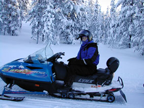
A famous example (slides 6 – 9) of his is the snowmobile. Conceptually, a snowmobile is a synthesis of skis, bicycle handles, outboard engine, and tank tread. Each item from disparate domains synthesized into a new capability. His discussion heuristically builds a foundation for this process from physics (Heisenberg), mathematics (Godel) and philosophy (Polanyi).

The key is that the process works reliably for conceptualization of ANYTHING: engineering artifacts, specific proposal contents, trade study candidates, strategies, etc. The concept pertains to non-engineering activities as well.

Snowmobile image used under GFDL with no implied endorsement

R. Pridham, DSP for Sonar

Roger Pridham and collaborators William Knight and Steven Kay document a comprehensive treatment of digital signal processing for sonar in a review article titled: Digital Signal Processing for Sonar, PROCEEDINGS OF THE IEEE, VOL. 69, NO. 11, NOVEMBER 1981. The article describes sonar processing from the water to the display. Pridham, et al., describe analog to digital conversion, filtering (analog and digital), detection, classification and localization (bearing and range estimation, Kalman tracking) and human interface. Active and passive sonar examples are worked out in detail to solidify the readers knowledge of the exposition. The hardware and software implementations discussed seem dated compared with the current state of the art for sonar. However, these do not detract and actually enhance understanding of legacy sonar applications.

One standout feature is a general formula for the beamwidth of a line array versus steering angle (IIB-57). The formula is approximate but more exact than most textbooks provide. The formula is good from broadside to endfire. The effect of aperture shading can be treated as a multiplicative factor (from Harris) on this equation. The formula can be applied to a two-dimensional panel array as an approximation (via a Mills cross equivalency). Finally, the formula is usable in an estimate of array directivity versus target angle.

Pridham identifies spatial transform processing as a form of beamforming along with the time delay and phase shift methods. The article also discusses adaptive beamforming and presents it in terms of bearing response (the power output of a beam scanned past a target). Another standout is the extensive discussion of digital sampling, complex spectra and aliasing. Perhaps most interesting is the date of the review, 1981. Many low-frequency active and passive sonars were digitized by this time. Studies were performed yearly documenting the current analog to digital conversion state of the art. Today, mid and higher frequency sonars are fully digital. At some point in the future, radio frequency communications and radar will realize the full impact of digitization.

F. Harris, On the Use of Windows…

This is a brief summary of a classic reference called “On the Use of Windows for Harmonic Analysis with the Discrete Fourier Transform” by Fredric J. Harris, PROCEEDINGS OF THE IEEE, VOL. 66, NO. 1, JANUARY 1978. Table 1 offers systems engineers the ability to quickly assess the effects of windowing on frequency, spatial or temporal transforms. In essence, windowing is a form of aperture filtering or shading that broadens a transform cell’s equivalent noise bandwidth, lowers the sidelobe level and, at 50% overlap, makes successive transforms almost independent (for “good” windows).

The paper describes many windows with desirable properties (and some with not so desirable ones). Several are easy to code for modeling purposes. Hanning is especially easy since, in the Fourier domain, its effects on a cell output are  the result of a phase weighted sum of that cell with the two adjacent Fourier cells. Dolph-Chebyshev has good properties: the narrowest mainlobe response for a given (uniform) sidelobe level. This window also has not so good properties, especially when used for spatial aperture shading of flexible arrays. The window exhibits a sidelobe suppression instability due to the alternating signs of its window coefficients.

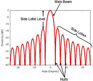
The results in Harris’ paper are useful for both systems analysis and design. The following figure from Wikipedia defines the main lobe (or beam), sidelobe level and sidelobes of a (continuous) transform response.